Note
Go to the end to download the full example code.
PyMieDiff + TorchGDM: Autodiff multi-scattering#
Multi‑particle scattering demo using PyMieDiff and TorchGDM.
- This script demonstrates how to:
Define a coated sphere (core + shell) with PyMieDiff.
Convert the particle to TorchGDM structures (full‑GPM and dipole‑only).
Run single‑particle extinction simulations and compare to Mie theory.
Visualise near‑field intensities for Mie, full‑GPM, and dipole models.
Set up a small cluster of identical particles, simulate with TorchGDM, and benchmark against a T‑matrix solution from the treams package.
Notes#
requires torchgdm: wiechapeter/torchgdm
requires treams: tfp-photonics/treams
TorchGDM paper: S. Ponomareva et al. SciPost Physics Codebases 60 (2025) doi: 10.21468/SciPostPhysCodeb.60
author: P. Wiecha, 11/2025
imports#
import time

import torch
import numpy as np
import matplotlib.pyplot as plt
from matplotlib.patches import Circle

import torchgdm as tg
import pymiediff as pmd
Mie particle config#
wl0 = torch.as_tensor([600, 700])
k0 = 2 * torch.pi / wl0

r_core = 150.0
r_shell = r_core + 100.0
n_core = 4.0
n_shell = 3.0
n_env = 1.0

mat_core = pmd.materials.MatConstant(n_core**2)
mat_shell = pmd.materials.MatConstant(n_shell**2)

# - setup the particle
particle = pmd.Particle(
    mat_env=n_env,
    r_core=r_core,
    mat_core=mat_core,
    r_shell=r_shell,
    mat_shell=mat_shell,
)
print(particle)


# convert to torchGDM structures
# dipole order only: fast, but inaccurate for large particles
structMieGPM_dp = pmd.helper.tg.StructAutodiffMieEffPola3D(particle, wavelengths=wl0)

# full multipole order: accurate, but slow model setup
structMieGPM_gpm = pmd.helper.tg.StructAutodiffMieGPM3D(
    particle, r_gpm=36, wavelengths=wl0
)
multilayer particle (on device: cpu)
 - layers   = 2
 - radii    = tensor([150., 250.])nm
 - materials: ['eps=16.00', 'eps=9.00']
 - environment    : eps=1.00

Extracting eff. dipole model from pymiediff...
/home/runner/work/MieDiff/MieDiff/src/pymiediff/helper/tg.py:864: UserWarning: Mie series: 1 wavelengths with significant residual electric quadrupole contribution: [np.float32(700.0)] nm
  warnings.warn(
/home/runner/work/MieDiff/MieDiff/src/pymiediff/helper/tg.py:875: UserWarning: Mie series: 2 wavelengths with significant residual magnetic quadrupole contribution: [np.float32(600.0), np.float32(700.0)] nm
  warnings.warn(
Done in 0.014s.
Extracting GPM model via pymiediff near-field eval...
   setup illuminations...

  0%|          | 0/2 [00:00<?, ?it/s]
GPM extraction:   0%|          | 0/2 [00:00<?, ?it/s]
GPM extraction: 100%|██████████| 2/2 [00:05<00:00,  2.60s/it]
Done in 6.8s.
torchGDM simulation#
# - illumination: normal incidence linear pol. plane wave
e_inc_list = [tg.env.freespace_3d.PlaneWave(e0p=1, e0s=0, inc_angle=0)]
env = tg.env.freespace_3d.EnvHomogeneous3D(env_material=n_env**2)

sim_single = tg.simulation.Simulation(
    structures=[structMieGPM_gpm],
    environment=env,
    illumination_fields=e_inc_list,
    wavelengths=wl0,
)
sim_single.run()

# extinction cross section comparison
cs_mie = particle.get_cross_sections(k0=k0)
cs = sim_single.get_spectra_crosssections()

print("")
print("Evaluated wavelengths (nm):")
print(f"     {wl0}")
print("PyMieDiff extinction cross section (nm^2):")
print(f"     {cs_mie["cs_ext"]}")
print("TorchGDM extinction cross section (nm^2):")
print(f"     {cs["ecs"][:,0]}")
print(f"rel. errors:")
print(f"     {[cs_mie["cs_ext"][i] / cs["ecs"][i] for i in range(len(wl0))]}")
------------------------------------------------------------
simulation on device 'cpu'...
 - homogeneous environment 3D
 - 1 structures
 - 36 positions
 - 72 coupled dipoles
   (of which 36 p, 36 m)
 - 2 wavelengths
 - 1 illumination fields per wavelength

run spectral simulation:

  0%|          | 0/2 [00:00<?, ?it/s]
  0%|          | 0/2 [00:00<?, ?it/s]
100%|██████████| 2/2 [00:00<00:00, 111.45it/s]
spectrum done in 0.02s
------------------------------------------------------------


  0%|          | 0/2 [00:00<?, ?it/s]
spectrum:   0%|          | 0/2 [00:00<?, ?it/s]
spectrum: 100%|██████████| 2/2 [00:00<00:00, 387.80it/s]

Evaluated wavelengths (nm):
     tensor([600, 700])
PyMieDiff extinction cross section (nm^2):
     tensor([253897.9303, 598618.8383], dtype=torch.float64)
TorchGDM extinction cross section (nm^2):
     tensor([253405.5000, 598822.9375])
rel. errors:
     [tensor([1.0019]), tensor([0.9997])]
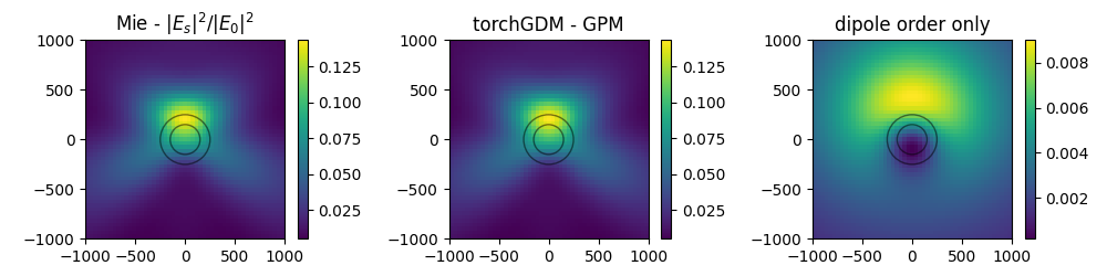
nearfield comparison#
single sphere : compare Mie theory and result for the torchGDM models
Note: the torchGDM models don’t support fields inside the particles, therefore we calculate fields in a plane next to the particles.
# also compare to dipole-approx. model
sim_single_dp = tg.simulation.Simulation(
    structures=[structMieGPM_dp],
    environment=env,
    illumination_fields=e_inc_list,
    wavelengths=wl0,
)
sim_single_dp.run()


# field calculation grid
projection = "xz"
r_probe = tg.tools.geometry.coordinate_map_2d_square(
    1000, 51, r3=500, projection=projection
)["r_probe"]

# which wavelength to plot
idx_wl = 0

# get nearfields
nf_mie = particle.get_nearfields(k0=k0[idx_wl], r_probe=r_probe)
nf_sim = sim_single.get_nearfield(wl0[idx_wl], r_probe=r_probe)
nf_sim_dp = sim_single_dp.get_nearfield(wl0[idx_wl], r_probe=r_probe)


# --- plot
def plot_circles(radii, pos=None, im=None):
    if pos is None:
        pos = [[0, 0]] * len(radii)

    for r, p in zip(radii, pos):
        rect = Circle(
            xy=p,
            radius=r,
            linewidth=1,
            edgecolor="k",
            facecolor="none",
            alpha=0.5,
        )
        plt.gca().add_patch(rect)
    if im is not None:
        cb = plt.colorbar(im, label="")


plt.figure(figsize=(10, 2.5))

# - Mie
plt.subplot(131, title="Mie - $|E_s|^2 / |E_0|^2$")
im = tg.visu2d.scalarfield(
    (torch.abs(nf_mie["E_s"]) ** 2).sum(-1),
    positions=r_probe,
    projection=projection,
)
clim = im.get_clim()
plot_circles([r_core, r_shell], im=im)

# - torchGDM - GPM
plt.subplot(132, title="torchGDM - GPM")
im = tg.visu2d.scalarfield(
    nf_sim["sca"].get_efield_intensity()[0],
    positions=r_probe,
    projection=projection,
)
im.set_clim(clim)
plot_circles([r_core, r_shell], im=im)

# - torchGDM - dipole order
plt.subplot(133, title="dipole order only")
im = tg.visu2d.scalarfield(
    nf_sim_dp["sca"].get_efield_intensity()[0],
    positions=r_probe,
    projection=projection,
)
plot_circles([r_core, r_shell], im=im)


plt.tight_layout()
plt.show()
------------------------------------------------------------
simulation on device 'cpu'...
 - homogeneous environment 3D
 - 1 structures
 - 1 positions
 - 2 coupled dipoles
   (of which 1 p, 1 m)
 - 2 wavelengths
 - 1 illumination fields per wavelength

run spectral simulation:

  0%|          | 0/2 [00:00<?, ?it/s]
  0%|          | 0/2 [00:00<?, ?it/s]
100%|██████████| 2/2 [00:00<00:00, 250.00it/s]
spectrum done in 0.01s
------------------------------------------------------------


  0%|          | 0/3 [00:00<?, ?it/s]
batched nearfield calculation:   0%|          | 0/3 [00:00<?, ?it/s]
batched nearfield calculation: 100%|██████████| 3/3 [00:00<00:00, 43.17it/s]

  0%|          | 0/3 [00:00<?, ?it/s]
batched nearfield calculation:   0%|          | 0/3 [00:00<?, ?it/s]
batched nearfield calculation: 100%|██████████| 3/3 [00:00<00:00, 247.36it/s]
multiple particles#
compare Mie theory and T-Matrix solver (treams)
# create simple multi-particle configuration: 5 particles on a circle
pos_multi = tg.tools.geometry.coordinate_map_1d_circular(r=700, n_phi=5)["r_probe"]

sim_multi = tg.simulation.Simulation(
    structures=[structMieGPM_gpm.copy(pos_multi)],
    environment=env,
    illumination_fields=e_inc_list,
    wavelengths=wl0,
)
sim_multi.run()

nf_sim_multi = sim_multi.get_nearfield(wl0[idx_wl], r_probe=r_probe)
------------------------------------------------------------
simulation on device 'cpu'...
 - homogeneous environment 3D
 - 1 structures
 - 180 positions
 - 360 coupled dipoles
   (of which 180 p, 180 m)
 - 2 wavelengths
 - 1 illumination fields per wavelength

run spectral simulation:

  0%|          | 0/2 [00:00<?, ?it/s]
  0%|          | 0/2 [00:00<?, ?it/s]
100%|██████████| 2/2 [00:00<00:00,  7.88it/s]
spectrum done in 0.26s
------------------------------------------------------------


  0%|          | 0/3 [00:00<?, ?it/s]
batched nearfield calculation:   0%|          | 0/3 [00:00<?, ?it/s]
batched nearfield calculation: 100%|██████████| 3/3 [00:00<00:00, 10.45it/s]
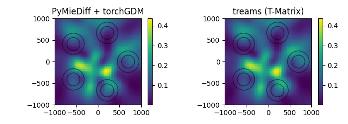
T-matrix multi-particle#
now we plot the nearfields in a plane parallel to the particle cluster and compare to the fields calculated with the treams T-matrix package.
Note: treams and GPM models do not support fields inside the particles, so we calculate fields outside of the particles.
import treams

t0 = time.time()

k0_treams = k0[idx_wl].cpu().numpy()

materials = [
    treams.Material(n_core**2),
    treams.Material(n_shell**2),
    treams.Material(n_env**2),
]
lmax = 5
spheres = [
    treams.TMatrix.sphere(lmax, k0_treams, [r_core, r_shell], materials)
    for i in range(len(pos_multi))
]
tm = treams.TMatrix.cluster(spheres, pos_multi.cpu().numpy()).interaction.solve()

e0_pol = [1, 0, 0]
inc = treams.plane_wave([0, 0, k0_treams], pol=e0_pol, k0=tm.k0, material=tm.material)
sca = tm @ inc.expand(tm.basis)

# calc nearfield
grid = r_probe.cpu().numpy()
e_sca_treams = sca.efield(grid)
e_inc_treams = inc.efield(grid)
e_tot_treams = e_sca_treams + e_inc_treams
intensity = np.sum(np.abs(e_sca_treams) ** 2, -1)

print("total time treams: {:.2f}s".format(time.time() - t0))
total time treams: 18.26s
plot the multi-particle nearfields#
plt.figure(figsize=(7, 2.5))

plt.subplot(121, title="PyMieDiff + torchGDM")
im = tg.visu2d.scalarfield(
    nf_sim_multi["sca"].get_efield_intensity()[0],
    positions=r_probe,
    projection=projection,
)
clim = im.get_clim()
plot_circles(
    len(pos_multi) * [r_core, r_shell],
    pos_multi[:, [0, 2]].repeat_interleave(2, dim=0),
    im=im,
)

plt.subplot(122, title="treams (T-Matrix)")
im = tg.visu2d.scalarfield(
    intensity,
    positions=r_probe,
    projection=projection,
)
im.set_clim(clim)
plot_circles(
    len(pos_multi) * [r_core, r_shell],
    pos_multi[:, [0, 2]].repeat_interleave(2, dim=0),
    im=im,
)

plt.tight_layout()
plt.show()
Automatic differentiation#
Now we can do any autodiff operation on a multi-particle simulation
Note: autodiff through GPM models is computationally relatively expensive as it requires back-propagation through a singular value decomposition. Consider using dipole-only models for small enough particles.
pmd.helper.tg.patch_torchgdm_autodiff()

wls = torch.as_tensor([600.0])
r_c_ad = torch.tensor(150.0, requires_grad=True)

# create some particles, one of which has a core radius requiring autograd
p1 = pmd.Particle(mat_env=1.0, r_core=r_c_ad, mat_core=3.5, r_shell=250, mat_shell=4.0)
gpm1 = pmd.helper.tg.StructAutodiffMieGPM3D(
    p1, r_gpm=36, wavelengths=wls, r0=[-500, 0, 0]
)

p2 = pmd.Particle(mat_env=1.0, r_core=100, mat_core=2.5, r_shell=120, mat_shell=1.5)
gpm2 = pmd.helper.tg.StructAutodiffMieGPM3D(
    p2, r_gpm=36, wavelengths=wls, r0=[500, 0, 0]
)

# combine structures without inplace ops to preserve autograd
combined_structures = pmd.helper.tg.combine_gpm_structures_autodiff(
    [gpm1, gpm2], environment=env
)

# create torchGDM simulation
sim_ad = tg.simulation.Simulation(
    structures=combined_structures,
    environment=env,
    illumination_fields=e_inc_list,
    wavelengths=wls,
    copy_structures=False,
)
sim_ad.run()

cs = sim_ad.get_spectra_crosssections()
t0 = time.time()
cs["ecs"][0].backward()

print("autograd finished in {:.1f}s".format(time.time() - t0))
print("d ECS / d r_core =", r_c_ad.grad)
Extracting GPM model via pymiediff near-field eval...
   setup illuminations...

  0%|          | 0/1 [00:00<?, ?it/s]
GPM extraction:   0%|          | 0/1 [00:00<?, ?it/s]
GPM extraction: 100%|██████████| 1/1 [00:03<00:00,  3.97s/it]
Done in 5.5s.
Extracting GPM model via pymiediff near-field eval...
   setup illuminations...

  0%|          | 0/1 [00:00<?, ?it/s]
GPM extraction:   0%|          | 0/1 [00:00<?, ?it/s]
GPM extraction: 100%|██████████| 1/1 [00:02<00:00,  2.32s/it]
Done in 3.5s.
/opt/hostedtoolcache/Python/3.12.13/x64/lib/python3.12/site-packages/torchgdm/struct/struct3d/gpm3d.py:99: UserWarning: Using different environment than specified in GPM-dict.
  warnings.warn("Using different environment than specified in GPM-dict.")
------------------------------------------------------------
simulation on device 'cpu'...
 - homogeneous environment 3D
 - 1 structures
 - 72 positions
 - 144 coupled dipoles
   (of which 72 p, 72 m)
 - 1 wavelengths
 - 1 illumination fields per wavelength

run spectral simulation:

  0%|          | 0/1 [00:00<?, ?it/s]
  0%|          | 0/1 [00:00<?, ?it/s]
100%|██████████| 1/1 [00:00<00:00, 72.74it/s]
spectrum done in 0.01s
------------------------------------------------------------


  0%|          | 0/1 [00:00<?, ?it/s]
spectrum:   0%|          | 0/1 [00:00<?, ?it/s]
spectrum: 100%|██████████| 1/1 [00:00<00:00, 342.22it/s]
autograd finished in 3.6s
d ECS / d r_core = tensor(-11321.4277)
Total running time of the script: (0 minutes 40.906 seconds)
Estimated memory usage: 1833 MB