getting started

demonstration of basic pymiediff functionality:

• Extinction, scattering and absorption spectra

• Angular scattering patterns

author: P. Wiecha, 03/2025

imports

import numpy as np
import torch
import matplotlib.pyplot as plt
from matplotlib.patches import Circle

import pymiediff as pmd

setup

we setup the particle dimension and materials as well as the environemnt. This is then wrapped up in an instance of Particle.

# - config
wl0 = torch.linspace(500, 1000, 100)
k0 = 2 * torch.pi / wl0

r_core = 70.0
r_shell = 100.0
mat_core = pmd.materials.MatDatabase("Si")
mat_shell = pmd.materials.MatDatabase("Ge")
n_env = 1.0

# - setup the particle
p = pmd.Particle(
    r_core=r_core,
    r_shell=r_shell,
    mat_core=mat_core,
    mat_shell=mat_shell,
    mat_env=n_env,
)
print(p)

core-shell particle
 - core radius    = 70.0nm
 - shell radius   = 100.0nm
 - core material  : Si
 - shell material : Ge
 - environment    : eps=1.00

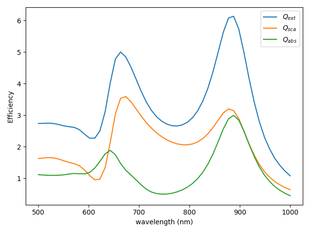
efficiency spectra

Calculate extinction, scattering and absorption spectra

cs = p.get_cross_sections(k0)

# - plot
plt.figure()
plt.plot(cs["wavelength"], cs["q_ext"], label="$Q_{ext}$")
plt.plot(cs["wavelength"], cs["q_sca"], label="$Q_{sca}$")
plt.plot(cs["wavelength"], cs["q_abs"], label="$Q_{abs}$")
plt.xlabel("wavelength (nm)")
plt.ylabel("Efficiency")
plt.legend()
plt.tight_layout()
# plt.savefig("ex_01a.svg", dpi=300)
plt.show()

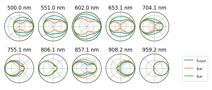
angular scattering

Calculate angular radiation patterns of the scattering

theta = torch.linspace(0.0, 2 * torch.pi, 100)
angular = p.get_angular_scattering(k0, theta)

# - plot every 10th wavelength
plt.figure(figsize=(7, 3))
for i, i_k0 in enumerate(range(len(k0))[::10]):
    ax = plt.subplot(2, 5, i + 1, polar=True)
    plt.title(f"{wl0[i_k0]:.1f} nm")
    ax.plot(angular["theta"], angular["i_unpol"][i_k0], label="$i_{unpol}$")
    ax.plot(angular["theta"], angular["i_par"][i_k0], label="$i_{par}$")
    ax.plot(angular["theta"], angular["i_per"][i_k0], label="$i_{per}$")
    ax.set_xticklabels([])
    ax.set_yticklabels([])
ax.legend(loc="center left", bbox_to_anchor=(1.4, 0.5))
plt.tight_layout()
# plt.savefig("ex_01b.svg", dpi=300)
plt.show()

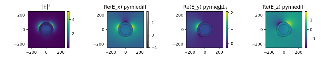
nearfields

Calculate nearfields in and around the partilce

# create grid of evaluation positions
d_area_plot = 250.0
x, z = torch.meshgrid(
    torch.linspace(-d_area_plot, d_area_plot, 100),
    torch.linspace(-d_area_plot, d_area_plot, 100),
)
y = torch.zeros_like(x)
grid = torch.stack([x, y, z], dim=-1)
orig_shape_grid = grid.shape

# evaluate the fields
i_wl = 15
fields_results = p.get_nearfields(k0=k0[i_wl], r_probe=grid.view(-1, 3))

# reshape fields to 2D grid
E_s = fields_results["E_s"]
E_s = E_s.view(orig_shape_grid)
intensity_sca_mie = torch.sum(E_s.abs() ** 2, dim=-1)


# --- plot
def plot_circles(radii, im=None):
    for r in radii:
        rect = Circle(
            xy=[0, 0],
            radius=r,
            linewidth=1.5,
            edgecolor="k",
            facecolor="C0",
            alpha=0.25,
        )
        plt.gca().add_patch(rect)
    if im is not None:
        cb = plt.colorbar(im, label="")


fig = plt.figure(figsize=(11, 2))
# - intensity
plt.subplot(141, aspect="equal", title="|E|$^2$")
im = plt.imshow(
    intensity_sca_mie.T,
    extent=(2 * (-d_area_plot, d_area_plot)),
    origin="lower",
)
plot_circles([r_core, r_shell], im)

# - field comp. (real part)
Ecomp_str = ["x", "y", "z"]
for i in range(3):
    plt.subplot(1, 4, i + 2, aspect="equal", title=f"Re(E_{Ecomp_str[i]}) pymiediff")
    im = plt.imshow(
        E_s[..., i].T.imag,
        extent=(2 * (-d_area_plot, d_area_plot)),
        origin="lower",
    )
    plot_circles([r_core, r_shell], im)

plt.tight_layout()
plt.show()

/opt/hostedtoolcache/Python/3.12.12/x64/lib/python3.12/site-packages/torch/functional.py:505: UserWarning: torch.meshgrid: in an upcoming release, it will be required to pass the indexing argument. (Triggered internally at /pytorch/aten/src/ATen/native/TensorShape.cpp:4317.)
  return _VF.meshgrid(tensors, **kwargs)  # type: ignore[attr-defined]

Estimated memory usage: 668 MB