Note
Go to the end to download the full example code.
particle optimisation#
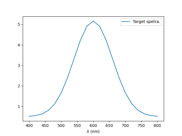
Demonstration of particle optimisation via gradient descent. Farfield cross sections are optimiatised to fit a guassian curve centered at 600.0nm.
Core and shell refractive indices and radii are optimised, with the materials limited to dispersionless dielectrics.
We optimize a large number of initial guesses concurrently, which avoids that a single solution gets stuck in a local minimum.
author: O. Jackson, P. Wiecha 03/2025
imports#
import time
import matplotlib.pyplot as plt
import pymiediff as pmd
import torch
import numpy as np

backend = "torch"
setup optimiation target#
# - define the range of wavelengths to be incuded in optimisation.
N_wl = 21
wl0 = torch.linspace(400, 800, N_wl)
k0 = 2 * torch.pi / wl0


# - for this example we target a gaussian like spectra centered at 600.0nm
def gaussian(x, mu, sig):
    return (
        1.0 / (np.sqrt(2.0 * np.pi) * sig) * np.exp(-np.power((x - mu) / sig, 2.0) / 2)
    )


target = gaussian(wl0.numpy(), 600.0, 60.0) * 700 + 0.5

target_tensor = torch.tensor(target)

# - we can plot the target spectra
plt.figure()
plt.plot(wl0, target, label="Target spetra.")
plt.xlabel("$\lambda$ (nm)")
plt.legend()
# plt.savefig("ex_04a.svg", dpi=300)
plt.show()
/home/runner/work/MieDiff/MieDiff/examples/ex_04_optimisation.py:53: SyntaxWarning: invalid escape sequence '\l'
  plt.xlabel("$\lambda$ (nm)")
setup particle prameter limits#
# - constants
n_env = 1.0

# - set limits to particle's properties, in this example we limit to dielectric materials
lim_r = torch.as_tensor([10, 100], dtype=torch.double)
lim_n_re = torch.as_tensor([1, 4.5], dtype=torch.double)
lim_n_im = torch.as_tensor([0, 0.1], dtype=torch.double)
normalization helper#
we let the optimizer work on normalized parameters which we pass through a sigmoid. This is a straightforward way to implement box boundaries for the optimization variables.
def params_to_physical(r_opt, n_opt):
    """converts normalised parameters to physical

    Args:
        r_opt (torch.Tensor): normalised radii
        n_opt (torch.Tensor): normalised materials

    Returns:
        torch.Tensor: physical parameters
    """

    # constrain optimization internally to physical limits
    # sigmoid: convert to [0, 1], then renormalize to physical limits
    sigmoid = torch.nn.Sigmoid()
    r_c_n, d_s_n = sigmoid(r_opt)
    n_c_re_n, n_s_re_n, n_c_im_n, n_s_im_n = sigmoid(n_opt)

    # scale parameters to physical units
    # size parameters
    r_c = r_c_n * (lim_r.max() - lim_r.min()) + lim_r.min()
    d_s = d_s_n * (lim_r.max() - lim_r.min()) + lim_r.min()
    r_s = r_c + d_s

    # core and shell complex ref. index
    n_c = (n_c_re_n * (lim_n_re.max() - lim_n_re.min()) + lim_n_re.min()) + 1j * (
        n_c_im_n * (lim_n_im.max() - lim_n_im.min()) + lim_n_im.min()
    )
    n_s = (n_s_re_n * (lim_n_re.max() - lim_n_re.min()) + lim_n_re.min()) + 1j * (
        n_s_im_n * (lim_n_im.max() - lim_n_im.min()) + lim_n_im.min()
    )

    return r_c, n_c**2, r_s, n_s**2
random initialization#
we use PyMieDiff’s vectorization capabilities to run the optimization of many random initial guesses in parallel.
# number of random guesses to make.
num_guesses = 100

# 2 size parameters (radius of core and thickness of shell)
# 4 material parameters: real and imag parts of constant ref. indices
r_opt_arr = torch.normal(0, 1, (2, num_guesses))
n_opt_arr = torch.normal(0, 1, (4, num_guesses))
r_opt_arr.requires_grad = True
n_opt_arr.requires_grad = True
optimisation loop#
define losses, create and run optimization loop. In this example adam optimizer is used, but the example is written such that it is ready to be used with LBFGS instead (requiring a “closure”).
max_iter = 50


# - define optimiser and hyperparameters
optimizer = torch.optim.AdamW(
    [r_opt_arr, n_opt_arr],
    lr=0.2,
)
# - alternative optimizer: LBFGS
# optimizer = torch.optim.LBFGS(
#     [r_opt_arr, n_opt_arr], lr=0.2, max_iter=10, history_size=7
# )


# - helper for batched forward pass (many particles)
def eval_batch(r_opt_arr, n_opt_arr):
    r_c, eps_c, r_s, eps_s = params_to_physical(r_opt_arr, n_opt_arr)

    # spectrally expand the permittivities
    eps_c = eps_c.unsqueeze(1).unsqueeze(1).broadcast_to(num_guesses, N_wl, 1)
    eps_s = eps_s.unsqueeze(1).unsqueeze(1).broadcast_to(num_guesses, N_wl, 1)

    # evaluate Mie
    result_mie = pmd.coreshell.cross_sections(
        k0.unsqueeze(0), r_c, eps_c, r_s, eps_s, backend=backend
    )["q_sca"]

    # get loss, MSE comparing target with current spectra
    losses = torch.mean(torch.abs(target_tensor.unsqueeze(0) - result_mie) ** 2, dim=1)

    return losses


# - required for LFBGS: closure (LFBGS calls f several times per iteration)
def closure():
    optimizer.zero_grad()  # Reset gradients

    losses = eval_batch(r_opt_arr, n_opt_arr)
    loss = torch.mean(losses)

    loss.backward()
    return loss


# - main loop
start_time = time.time()
loss_hist = []  # Array to store loss data
for o in range(max_iter + 1):

    loss = optimizer.step(closure)  # LBFGS requires closure
    all_losses = eval_batch(r_opt_arr, n_opt_arr)
    loss_hist.append(loss.item())  # Store loss value

    if o % 1 == 0:
        i_best = torch.argmin(all_losses)
        r_c, eps_c, r_s, eps_s = params_to_physical(r_opt_arr, n_opt_arr)
        print(
            " --- iter {}: loss={:.2f}, best={:.2f}".format(
                o, loss.item(), all_losses.min().item()
            )
        )
        print(
            "     r_core, r_shell  = {:.1f}nm,     {:.1f}nm".format(
                r_c[i_best], r_s[i_best]
            )
        )
        print(
            "     n_core, n_shell  = {:.2f}, {:.2f}".format(
                torch.sqrt(eps_c[i_best]), torch.sqrt(eps_s[i_best])
            )
        )

# - finished
print(50 * "-")
t_opt = time.time() - start_time
print(
    "Optimization finished in {:.1f}s ({:.1f}s per iteration)".format(
        t_opt, t_opt / max_iter
    )
)
 --- iter 0: loss=4.85, best=0.39
     r_core, r_shell  = 74.6nm,     112.7nm
     n_core, n_shell  = 3.79+0.04j, 1.79+0.07j
 --- iter 1: loss=3.67, best=0.42
     r_core, r_shell  = 59.6nm,     116.9nm
     n_core, n_shell  = 3.99+0.08j, 2.08+0.08j
 --- iter 2: loss=3.17, best=0.70
     r_core, r_shell  = 63.8nm,     137.4nm
     n_core, n_shell  = 3.83+0.07j, 1.79+0.02j
 --- iter 3: loss=2.89, best=0.43
     r_core, r_shell  = 62.4nm,     119.1nm
     n_core, n_shell  = 4.30+0.04j, 1.73+0.03j
 --- iter 4: loss=2.67, best=0.40
     r_core, r_shell  = 74.2nm,     113.6nm
     n_core, n_shell  = 3.82+0.05j, 1.68+0.08j
 --- iter 5: loss=2.40, best=0.44
     r_core, r_shell  = 64.4nm,     123.8nm
     n_core, n_shell  = 4.21+0.05j, 1.70+0.05j
 --- iter 6: loss=2.21, best=0.32
     r_core, r_shell  = 68.0nm,     104.5nm
     n_core, n_shell  = 4.10+0.08j, 2.09+0.07j
 --- iter 7: loss=2.09, best=0.40
     r_core, r_shell  = 62.5nm,     119.7nm
     n_core, n_shell  = 4.05+0.09j, 1.95+0.08j
 --- iter 8: loss=1.99, best=0.46
     r_core, r_shell  = 65.4nm,     111.5nm
     n_core, n_shell  = 3.81+0.09j, 2.27+0.08j
 --- iter 9: loss=1.86, best=0.34
     r_core, r_shell  = 64.8nm,     110.1nm
     n_core, n_shell  = 3.87+0.09j, 2.22+0.08j
 --- iter 10: loss=1.74, best=0.34
     r_core, r_shell  = 64.2nm,     108.7nm
     n_core, n_shell  = 3.92+0.09j, 2.17+0.08j
 --- iter 11: loss=1.68, best=0.32
     r_core, r_shell  = 68.6nm,     106.4nm
     n_core, n_shell  = 4.15+0.09j, 1.98+0.08j
 --- iter 12: loss=1.63, best=0.31
     r_core, r_shell  = 64.2nm,     108.1nm
     n_core, n_shell  = 4.02+0.09j, 2.10+0.08j
 --- iter 13: loss=1.54, best=0.26
     r_core, r_shell  = 64.9nm,     108.7nm
     n_core, n_shell  = 4.06+0.09j, 2.09+0.08j
 --- iter 14: loss=1.46, best=0.27
     r_core, r_shell  = 65.5nm,     109.5nm
     n_core, n_shell  = 4.10+0.09j, 2.08+0.09j
 --- iter 15: loss=1.39, best=0.29
     r_core, r_shell  = 66.0nm,     109.9nm
     n_core, n_shell  = 4.13+0.09j, 2.07+0.09j
 --- iter 16: loss=1.34, best=0.28
     r_core, r_shell  = 65.6nm,     117.2nm
     n_core, n_shell  = 4.22+0.03j, 1.78+0.03j
 --- iter 17: loss=1.29, best=0.26
     r_core, r_shell  = 60.3nm,     110.3nm
     n_core, n_shell  = 4.21+0.10j, 2.23+0.09j
 --- iter 18: loss=1.23, best=0.23
     r_core, r_shell  = 59.8nm,     109.1nm
     n_core, n_shell  = 4.22+0.10j, 2.21+0.09j
 --- iter 19: loss=1.18, best=0.22
     r_core, r_shell  = 56.5nm,     105.8nm
     n_core, n_shell  = 4.29+0.09j, 2.37+0.09j
 --- iter 20: loss=1.14, best=0.25
     r_core, r_shell  = 56.3nm,     105.1nm
     n_core, n_shell  = 4.30+0.09j, 2.34+0.09j
 --- iter 21: loss=1.09, best=0.23
     r_core, r_shell  = 59.8nm,     107.5nm
     n_core, n_shell  = 4.17+0.09j, 2.27+0.08j
 --- iter 22: loss=1.06, best=0.22
     r_core, r_shell  = 60.4nm,     107.9nm
     n_core, n_shell  = 4.31+0.09j, 2.17+0.09j
 --- iter 23: loss=1.02, best=0.20
     r_core, r_shell  = 57.4nm,     105.9nm
     n_core, n_shell  = 4.33+0.09j, 2.31+0.09j
 --- iter 24: loss=0.99, best=0.20
     r_core, r_shell  = 58.1nm,     106.6nm
     n_core, n_shell  = 4.34+0.09j, 2.31+0.09j
 --- iter 25: loss=0.95, best=0.20
     r_core, r_shell  = 60.9nm,     104.9nm
     n_core, n_shell  = 4.34+0.09j, 2.21+0.10j
 --- iter 26: loss=0.92, best=0.21
     r_core, r_shell  = 61.4nm,     104.8nm
     n_core, n_shell  = 4.34+0.09j, 2.23+0.10j
 --- iter 27: loss=0.89, best=0.21
     r_core, r_shell  = 58.8nm,     106.8nm
     n_core, n_shell  = 4.36+0.09j, 2.29+0.09j
 --- iter 28: loss=0.84, best=0.18
     r_core, r_shell  = 55.6nm,     104.3nm
     n_core, n_shell  = 4.45+0.10j, 2.41+0.10j
 --- iter 29: loss=0.82, best=0.18
     r_core, r_shell  = 55.7nm,     102.8nm
     n_core, n_shell  = 4.45+0.10j, 2.40+0.10j
 --- iter 30: loss=0.82, best=0.18
     r_core, r_shell  = 56.1nm,     101.9nm
     n_core, n_shell  = 4.45+0.10j, 2.40+0.10j
 --- iter 31: loss=0.81, best=0.17
     r_core, r_shell  = 56.9nm,     101.8nm
     n_core, n_shell  = 4.45+0.10j, 2.41+0.10j
 --- iter 32: loss=0.79, best=0.17
     r_core, r_shell  = 57.7nm,     101.8nm
     n_core, n_shell  = 4.45+0.10j, 2.42+0.10j
 --- iter 33: loss=0.76, best=0.18
     r_core, r_shell  = 58.2nm,     101.5nm
     n_core, n_shell  = 4.46+0.10j, 2.42+0.10j
 --- iter 34: loss=0.74, best=0.17
     r_core, r_shell  = 58.3nm,     100.6nm
     n_core, n_shell  = 4.46+0.10j, 2.42+0.10j
 --- iter 35: loss=0.72, best=0.18
     r_core, r_shell  = 58.2nm,     99.7nm
     n_core, n_shell  = 4.46+0.10j, 2.42+0.10j
 --- iter 36: loss=0.70, best=0.19
     r_core, r_shell  = 58.3nm,     99.2nm
     n_core, n_shell  = 4.46+0.10j, 2.42+0.10j
 --- iter 37: loss=0.68, best=0.18
     r_core, r_shell  = 57.0nm,     106.0nm
     n_core, n_shell  = 4.45+0.06j, 2.28+0.09j
 --- iter 38: loss=0.66, best=0.17
     r_core, r_shell  = 56.6nm,     104.0nm
     n_core, n_shell  = 4.46+0.09j, 2.35+0.10j
 --- iter 39: loss=0.65, best=0.18
     r_core, r_shell  = 57.6nm,     99.4nm
     n_core, n_shell  = 4.42+0.10j, 2.50+0.10j
 --- iter 40: loss=0.63, best=0.18
     r_core, r_shell  = 56.9nm,     102.1nm
     n_core, n_shell  = 4.46+0.09j, 2.36+0.10j
 --- iter 41: loss=0.61, best=0.17
     r_core, r_shell  = 57.4nm,     101.9nm
     n_core, n_shell  = 4.46+0.09j, 2.37+0.10j
 --- iter 42: loss=0.59, best=0.17
     r_core, r_shell  = 58.0nm,     102.0nm
     n_core, n_shell  = 4.46+0.09j, 2.39+0.10j
 --- iter 43: loss=0.59, best=0.17
     r_core, r_shell  = 57.8nm,     100.8nm
     n_core, n_shell  = 4.42+0.10j, 2.45+0.10j
 --- iter 44: loss=0.59, best=0.18
     r_core, r_shell  = 57.6nm,     100.7nm
     n_core, n_shell  = 4.42+0.10j, 2.43+0.10j
 --- iter 45: loss=0.58, best=0.17
     r_core, r_shell  = 58.3nm,     100.5nm
     n_core, n_shell  = 4.46+0.09j, 2.40+0.10j
 --- iter 46: loss=0.57, best=0.18
     r_core, r_shell  = 58.2nm,     102.4nm
     n_core, n_shell  = 4.41+0.10j, 2.40+0.10j
 --- iter 47: loss=0.55, best=0.17
     r_core, r_shell  = 56.3nm,     102.5nm
     n_core, n_shell  = 4.46+0.10j, 2.41+0.10j
 --- iter 48: loss=0.54, best=0.17
     r_core, r_shell  = 57.9nm,     102.1nm
     n_core, n_shell  = 4.42+0.10j, 2.40+0.10j
 --- iter 49: loss=0.53, best=0.17
     r_core, r_shell  = 57.9nm,     99.7nm
     n_core, n_shell  = 4.46+0.10j, 2.44+0.10j
 --- iter 50: loss=0.52, best=0.17
     r_core, r_shell  = 57.4nm,     101.2nm
     n_core, n_shell  = 4.46+0.10j, 2.44+0.10j
--------------------------------------------------
Optimization finished in 3.0s (0.1s per iteration)
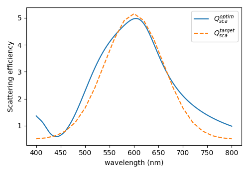
optimisation results#
view optimised speactra and corresponding particle parameters.
# - plot optimised spectra against target spectra
wl0_eval = torch.linspace(400, 800, 200)
k0_eval = 2 * torch.pi / wl0_eval

i_best = torch.argmin(all_losses)
r_c, eps_c, r_s, eps_s = params_to_physical(r_opt_arr[:, i_best], n_opt_arr[:, i_best])

cs_opt = pmd.coreshell.cross_sections(k0_eval, r_c, eps_c, r_s, eps_s)

plt.figure(figsize=(5, 3.5))
plt.plot(cs_opt["wavelength"], cs_opt["q_sca"][0].detach(), label="$Q_{sca}^{optim}$")
plt.plot(wl0, target_tensor, label="$Q_{sca}^{target}$", linestyle="--")
plt.xlabel("wavelength (nm)")
plt.ylabel("Scattering efficiency")
plt.legend()
plt.tight_layout()
plt.show()


# - print optimun parameters
print(50 * "-")
print("optimum:")
print(" r_core  = {:.1f}nm".format(r_c))
print(" r_shell = {:.1f}nm".format(r_s))
print(" n_core  = {:.2f}".format(torch.sqrt(eps_c)))
print(" n_shell = {:.2f}".format(torch.sqrt(eps_s)))
--------------------------------------------------
optimum:
 r_core  = 57.4nm
 r_shell = 101.2nm
 n_core  = 4.46+0.10j
 n_shell = 2.44+0.10j
Total running time of the script: (0 minutes 5.298 seconds)
Estimated memory usage: 778 MB